Creating an interactive 3D terrain model of an idyllic Wisconsin river town with Rayshader in R

3D terrain models are fascinating to experiment with, and R’s rayshader package makes it shockingly simple to produce them in just a few lines of code. In this post, I’ll demonstrate how to (a) retrieve publicly accessible terrain data for the state of Wisconsin, (b) crop that dataset to municipality boundaries using US Census TIGER files, and (c) create the interactive 3D terrain model.

First, we load necessary packages and set desired options:

library(terra)
library(tigris)
library(dplyr)
library(here)
library(sf)
library(tmap)
library(rayshader)

tmap_mode("view")

terra is used for reading raster datasets (and other raster data operations)
tigris is used for retrieving US Census TIGER files (in our case, “places”)
dplyr is used for manipulation
here is used for file system operations using relative paths (crucial for reproducibiltiy across machines)
sf is used for vector spatial operations
tmap is used for mapping vector data
rayshader is used for 3D visualizations

Setting tmap_mode to “view” ensures that tmap always creates a web for us. I prefer this to static maps since it allows us to see context and explore the data in a bit more detail.

Next, we need to download data. The terrain data is a digital elevation model (DEM) dataset that comes from the Wisconsin DNR, and this step is surprisingly difficult to make reproducible. The necessary dataset is served by the DNR here, but the format is somewhat clunky. Opening that webpage takes one to the documentation page for the dataset and also triggers an immediate download. Unfortunately we cannot download the dataset directly using the terminal utility wget since that just retrieves the web page content instead of the dataset itself. To mitigate this – and since I utilize this DEM often – I have a copy of the zipped file available in a publicly hosted git repository that can be downloaded directly with wget.

fname <- here("data-raw", "DEM_30m.zip")

cmd_dl <- paste("wget -O",
                 fname,
                "https://gitlab.com/mhaffner/data/-/raw/master/DEM_30m.zip?ref_type=heads&inline=false",
                "&")

cmd_unzip <- paste("unzip",
                   here("data-raw/DEM_30m.zip"),
                   "-d",
                   here("data-raw"))

system(cmd_dl)
system(cmd_unzip)

It’s quite possible that this is more work than it’s worth, but I’m obsessed with reproducibiltiy, and it’s also quite possible that some grad student somewhere will thank me for using relative paths and direct downloads, so this is a chance I’m willing to take. It should be noted that you would likely want to .gitignore the DEM files; otherwise it’ll take forever to push/pull to a version controlled repo. In my blogdown sites, I simply just ignore the entire data-raw directory. Then, we can read the raster dataset directly:

wi_dem <- rast(here("data-raw/DEM_30m/demgw930"))

We can create a quick plot to verify the dataset with the plot method:

plot(wi_dem)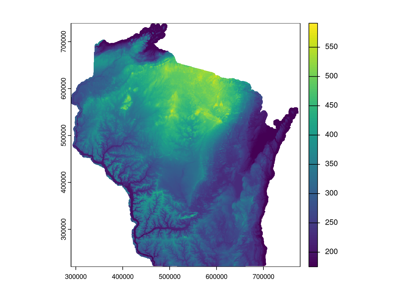

Next, we’ll collect data on municipal boundaries for all Wisconsin towns and subset it to my new favorite Mississippi River town, Fountain City:

wi_places <- places(state = "WI", progress_bar = FALSE) %>%
  st_transform(st_crs(wi_dem))

fc <- wi_places %>%
  filter(NAME == "Fountain City")

Since we want this dataset to play nicely with our DEM, we transform data into that of the CRS of the DEM (in part because census data uses a geographic CRS, EPSG:4269). We can then create a simple web map of the location, making it 90% transparent:

tm_shape(fc) +
  tm_basemap("Esri.WorldTopoMap") +
  tm_polygons(fill = "blue",
              fill_alpha = 0.1)

Then, we crop the raster to that of the DEM and create another quick visualization:

fc_dem <- crop(wi_dem, fc)
plot(fc_dem)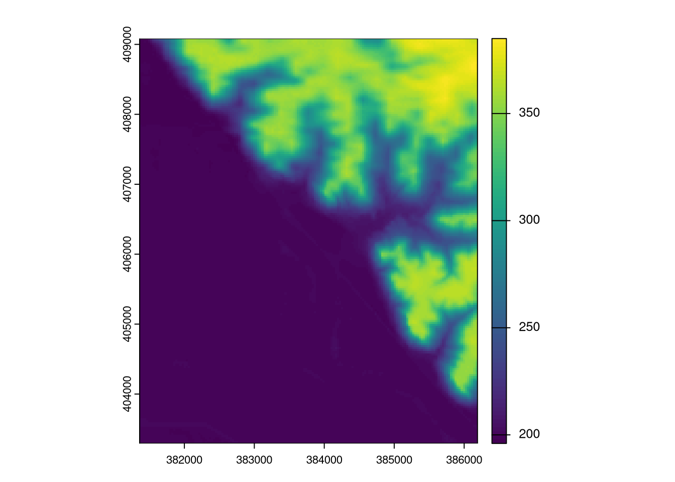

rayshader needs a matrix rather than a true raster dataset, so we create one with the function, raster_to_matrix (it’s almost so easy that it’s not fair):

fc_mat <- raster_to_matrix(fc_dem)

Years ago I had undertaken this process with the now defunct raster package, but fortunately almost all of the functions in R’s next generation raster data handler, terra were word-for-word (or nearly word-for-word) identical and also return objects of similar structure. If only all package transitions could go this smoothly.

Next, we can create a simple 2D visualization with rayshader, detecting water directly from the dataset itself:

fc_mat %>%
  sphere_shade(texture = "imhof1") %>%
  add_water(detect_water(fc_mat)) %>%
  plot_map()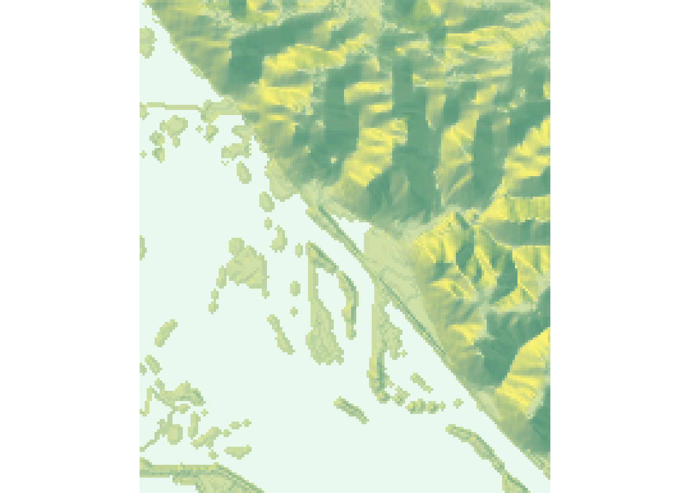

This also adds some shading and uses a terrain-like texture. Finally, we’re able to create a 3D visualization, again detecting water but also adding shadows. We can adjust view parameters with fov, theta, zoom, and phi along with exaggerating elevation a bit with the zscale argument. Since summer is lasting a little too long at the moment (I’ll eat these words come mid April), we’ll speed the seasons along by using a terrain texture that is slightly less verdant:

fc_mat %>%
  sphere_shade(texture = "imhof4") %>%
  add_water(detect_water(fc_mat), color = "imhof4") %>%
  add_shadow(ray_shade(fc_mat, zscale = 8), 0.5) %>%
  add_shadow(ambient_shade(fc_mat), 0) %>%
  plot_3d(fc_mat, zscale = 25, fov = 0, theta = 345, zoom = 0.75, phi = 25)

rgl::rglwidget()

It’s interactive! So zoom in and out, and pan around to change the view!

Getting the interactive version to appear in an RMarkdown file requires the use of rgl and rglwidget, which is the only additional step needed if not running the code interactively. The wonderful thing about this approach is that it will work with any Wisconsin town simply by changing the input to the NAME argument utilized in subsetting the places dataset. One word of caution, however: rayshader is computationally intensive, and it will take significantly more time to create an interactive visualization of larger (in terms of land area) towns. This can be mitigated by resampling the raster down to make it more manageable.

It’s amazing how far R has come in it’s 3D terrain visualization capabilities. Tyler Morgan-Wall (creator of rayshader) is in large part to thank for this. Five years ago I was creating similar visualizations with rgl, but the outputs were artificial looking, computations took an eon, and there wasn’t an efficient way to embed the interactive outputs in an RMarkdown document. Now all this is much simpler, and it feels like I’m living in a dream! From top to bottom, this script takes about 15 seconds to run on my 8 year old home desktop, including downloading and unzipping files, creating the web map, and producing all rayshader outputs. What a wonderful world.