This short post provides an overview of my typical workflow when working with
regression models. I think it is helpful to start with a simple example first
(i.e. bivariate OLS) and work toward more complex examples. The syntax for OLS
is a bit easier to understand, yet model construction translates well to more
complex forms. In this example I’ll use one of the datasets from the ggplot2
library, mpg.
Exploratory data analysis
The mpg dataset contains a number of variables including the manufacturer
(mpg$manufactur), engine displacement (mpg$displ), number of cylinders
(mpg$cyl), miles per gallon when driving in the city (mpg$cty), and miles
per gallon when driving on the highway (mpg$hwy). We can get some information
about the dataset with the following:
library(ggplot2)

## view the contents
mpg
## # A tibble: 234 × 11
## manufacturer model displ year cyl trans drv cty hwy fl class
## <chr> <chr> <dbl> <int> <int> <chr> <chr> <int> <int> <chr> <chr>
## 1 audi a4 1.8 1999 4 auto… f 18 29 p comp…
## 2 audi a4 1.8 1999 4 manu… f 21 29 p comp…
## 3 audi a4 2 2008 4 manu… f 20 31 p comp…
## 4 audi a4 2 2008 4 auto… f 21 30 p comp…
## 5 audi a4 2.8 1999 6 auto… f 16 26 p comp…
## 6 audi a4 2.8 1999 6 manu… f 18 26 p comp…
## 7 audi a4 3.1 2008 6 auto… f 18 27 p comp…
## 8 audi a4 quattro 1.8 1999 4 manu… 4 18 26 p comp…
## 9 audi a4 quattro 1.8 1999 4 auto… 4 16 25 p comp…
## 10 audi a4 quattro 2 2008 4 manu… 4 20 28 p comp…
## # … with 224 more rowsOr, for a little more flexibility we can use the datatable function from the DT
library to create an interactive table:
library(DT)

datatable(mpg)
If we’re interested in only a few of these components, we can use some of the functions below. The output is hidden here since much of it is redundant.
## number of rows
nrow(mpg)

## number of columns
ncol(mpg)

## names of columns
names(mpg)

## view metadata, only useful for a built-in dataset though
?mpg

## view the unique values of a column, useful for categorical data
unique(mpg$manufacturer)
OLS
Suppose we are interested in the relationship between engine displacement
(mpg$displ) and miles per gallon when driving on the highway (mpg$hwy). We
expect a negative relationship and we can explore this with the base plot
function:
plot(mpg$displ, mpg$hwy)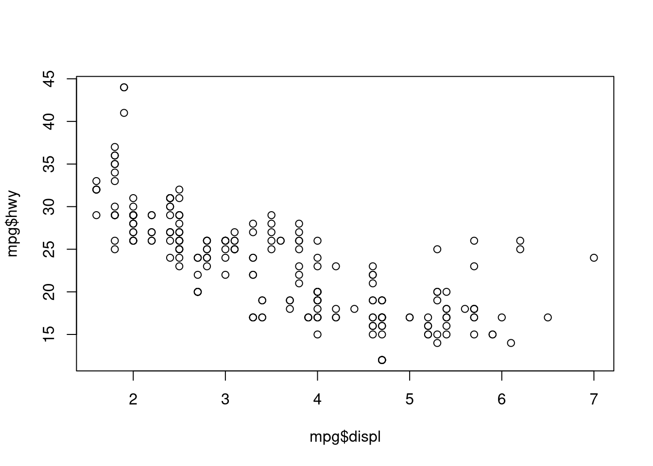
Or for a more sophisticated plot that is perhaps a bit more publication worthy:
ggplot(data = mpg,
       aes(displ, hwy)) +
  geom_point()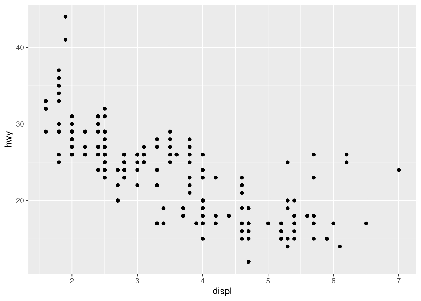
I think this is a good example for a polynomial regression problem because a linear function will work pretty well, but a polynomial function will likely be better.
Of course, when conducting regression it can be useful to explore characteristics of the individual variables:
## set plot parameters; one row and two column (to get figures side by side)
par(mfrow = c(1, 2))

hist(mpg$displ)
hist(mpg$hwy)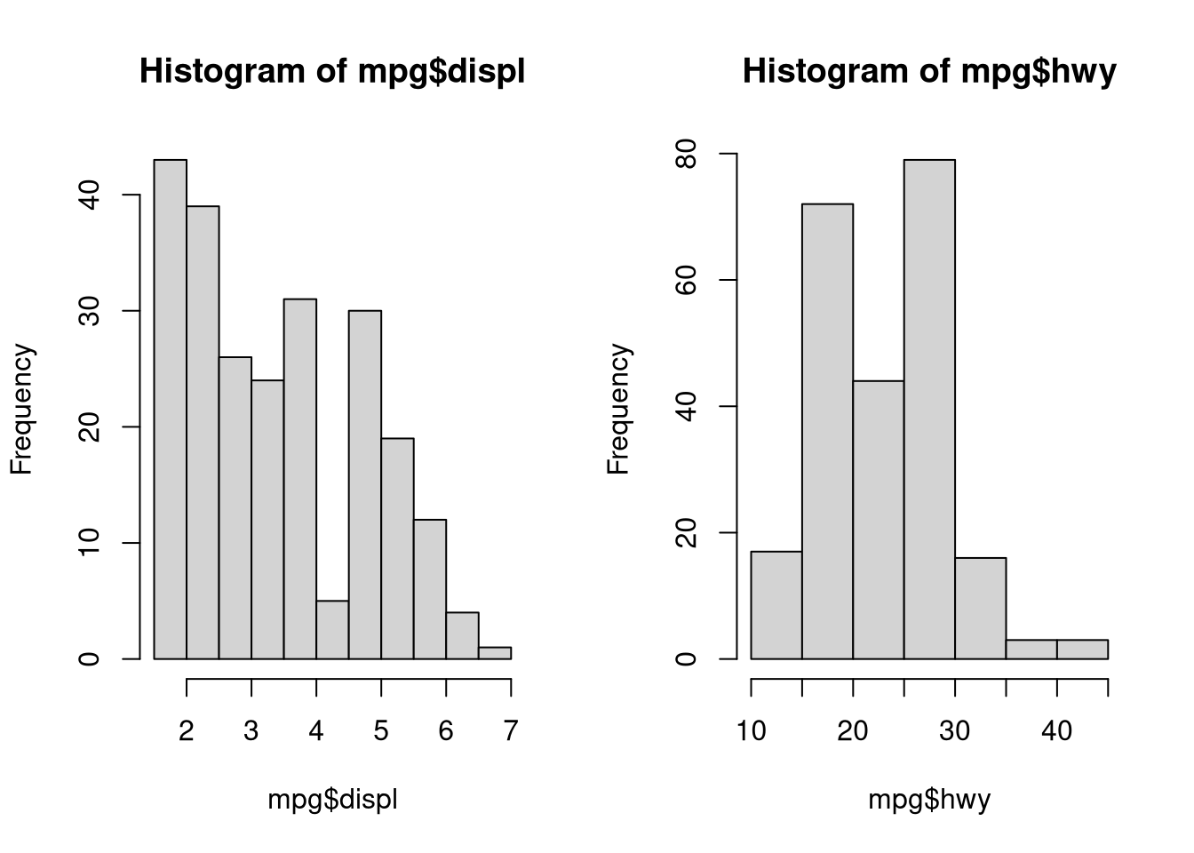
…and a more sophisticated plot:
library(gridExtra)

## engine displacment histogram
displ.hist <- ggplot(data = mpg,
                     aes(displ)) +
  geom_histogram(bins = 10)

## highway miles per gallon histogram
hwy.hist <- ggplot(data = mpg,
       aes(hwy)) +
  geom_histogram(bins = 10)

## place plots side by side
grid.arrange(displ.hist, hwy.hist, nrow = 1)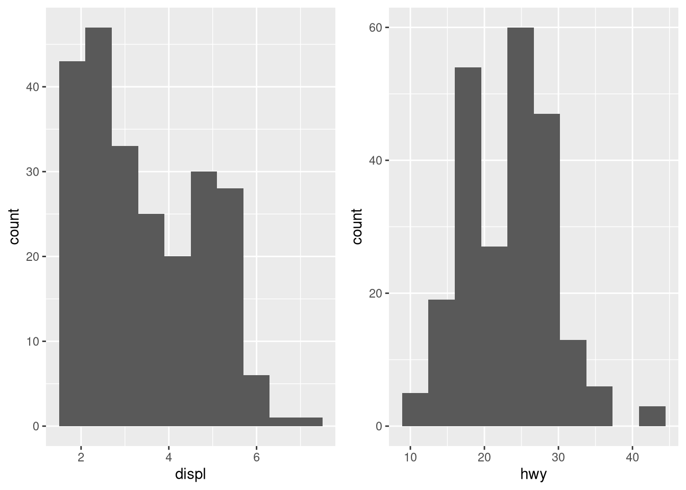
Clearly the x variable may pose problems, but let’s move on. To actually
complete the linear regression model, we can use the lm function which is a
base R function. In the lm call above, I like to think of replacing the ~
operator with the phrase “as a function of…” In this case, hwy is a function
of displ.
## we don't have to put the result in a variable but it gives us access to more information.
ols.model.1 <- lm(hwy ~ displ,
                data = mpg)

## view the results
ols.model.1
##
## Call:
## lm(formula = hwy ~ displ, data = mpg)
##
## Coefficients:
## (Intercept) displ
## 35.698 -3.531## get some more detailed information
summary(ols.model.1)##
## Call:
## lm(formula = hwy ~ displ, data = mpg)
##
## Residuals:
## Min 1Q Median 3Q Max
## -7.1039 -2.1646 -0.2242 2.0589 15.0105
##
## Coefficients:
## Estimate Std. Error t value Pr(>|t|)
## (Intercept) 35.6977 0.7204 49.55 <0.0000000000000002 ***
## displ -3.5306 0.1945 -18.15 <0.0000000000000002 ***
## ---
## Signif. codes: 0 '***' 0.001 '**' 0.01 '*' 0.05 '.' 0.1 ' ' 1
##
## Residual standard error: 3.836 on 232 degrees of freedom
## Multiple R-squared: 0.5868, Adjusted R-squared: 0.585
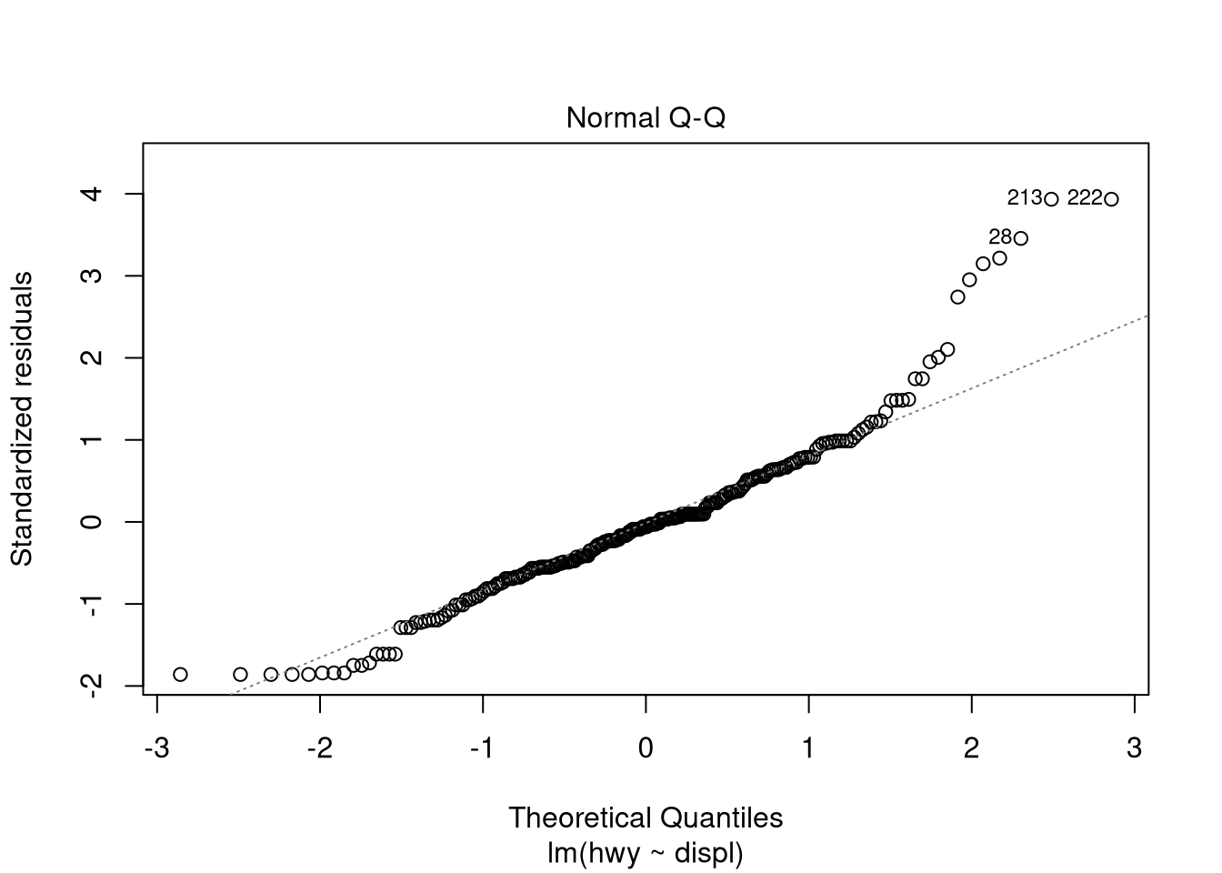
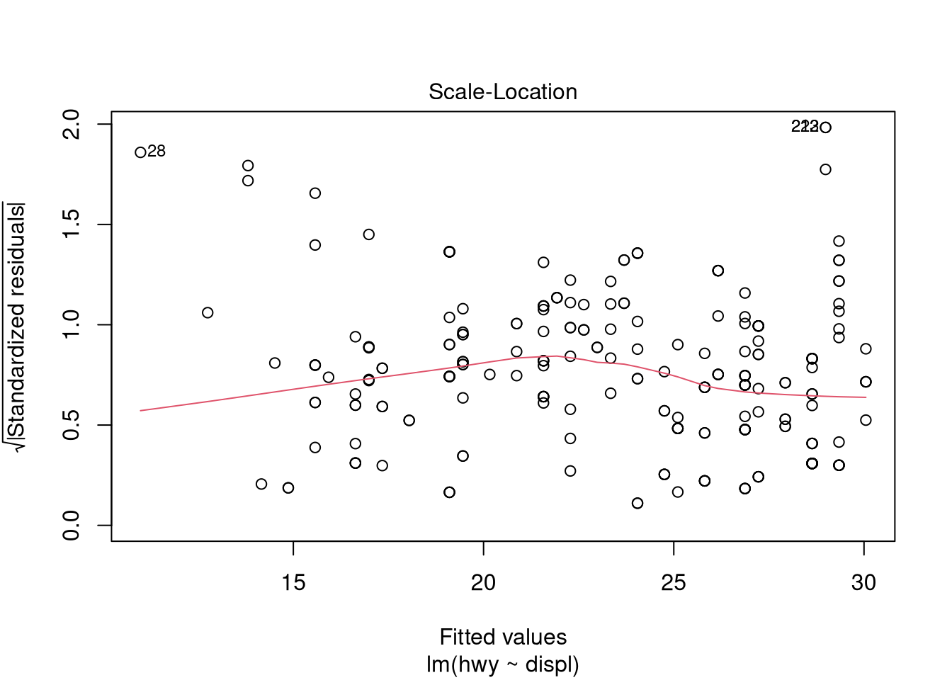
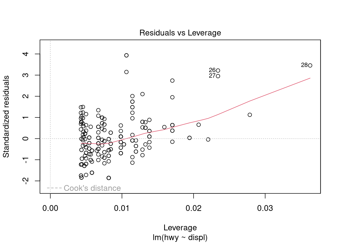
## F-statistic: 329.5 on 1 and 232 DF, p-value: < 0.00000000000000022Use graphical measures to evaluate the model:
plot(ols.model.1)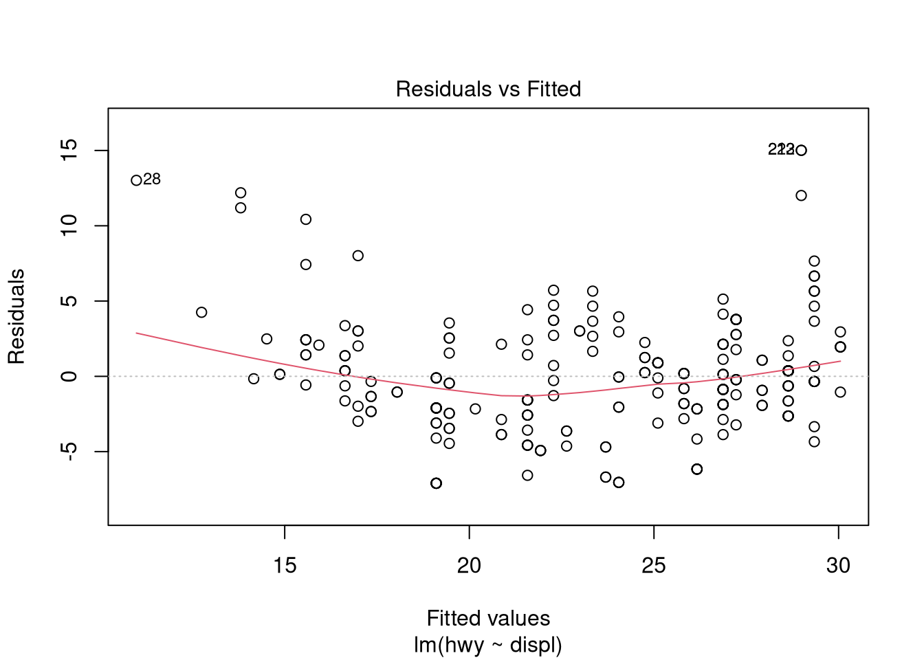
Plot the actual vs. fitted values:
plot(mpg$displ, mpg$hwy)
abline(ols.model.1)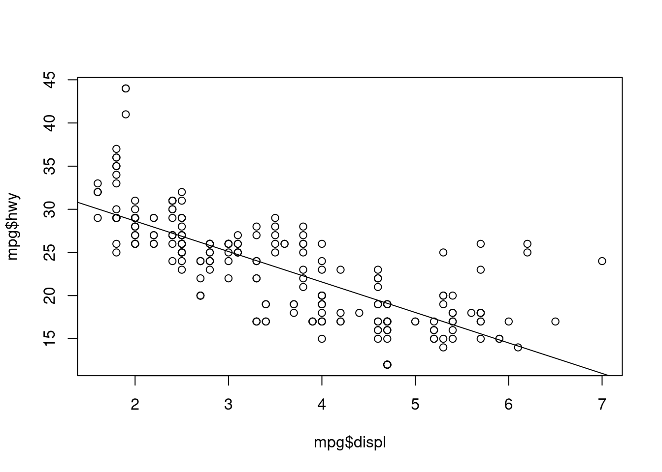
We can evaluate the assumption of residual normality with graphical measures…
hist(ols.model.1$residuals)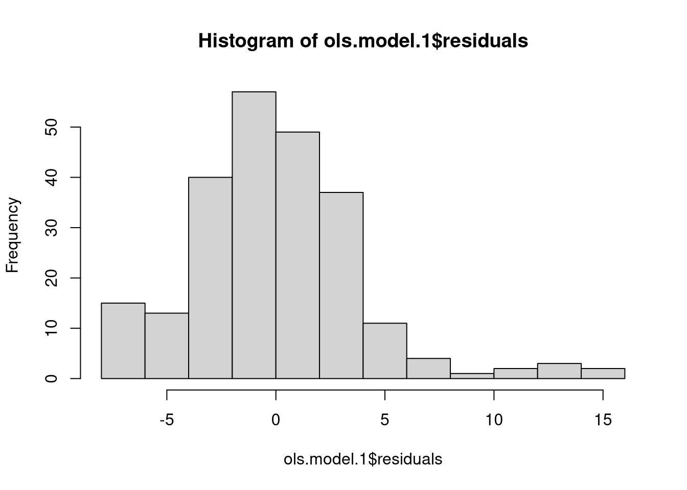
…and/or with a test
shapiro.test(ols.model.1$residuals)##
## Shapiro-Wilk normality test
##
## data: ols.model.1$residuals
## W = 0.94125, p-value = 0.00000004343Adding more variables to the regression model is easy; just use the + operator
in the function call. Here, highway miles per gallon is a function of engine
displacement (displ), whether or not the car is an SUV (manually created
dummay variable, suv), and number of cylinders (cyl).
## create a dummy variable for SUVs
mpg$suv <- 0
mpg[mpg$class == "suv",]$suv <- 1

## new model
ols.model.2 <- lm(hwy ~ displ +
                    suv +
                    cyl,
                  data = mpg,)
There are different ways to evaluate VIF, but the car library has a
straightforward function: vif.
library(car)

## some significant multicollinearity here
vif(ols.model.2)
## displ suv cyl
## 7.918850 1.273033 7.464803Variable transformations and polynomial regression
Before demonstrating polynomial regression, it’s worth pointing out that
variables can be manually transformed within the function call. These particular
transformations don’t necessarily make sense here, but it demonstrates the idea.
To use arithmetic operators within the function call, the I function needs to
precede the operation. This means interpret “as is”. E.g.,
## new model with transformations
trans.model.1 <- lm(hwy ~ log(displ) +
                    suv +
                    I(1/cyl),
                  data = mpg,)
This is not necessary with log since it is a built-in function whereas \ is
an operator. Or just transform the variables outside of the function call:
## log of engine displacement
mpg$log.displ <- log(mpg$displ)

## 1 over number of cylinders
mpg$inv.cyl <- 1/mpg$cyl

## new model with transformations
trans.model.2 <- lm(hwy ~ log.displ +
                    suv +
                    inv.cyl,
                  data = mpg,)
There are a few different options for polynomial regression. Let’s return to the
original example with only two variables: hwy and displ. Similar to the
method above, we can transform variables to any degree we want within the
function call:
## univariate polynomial regression
poly.model.1 <- lm(hwy ~ displ + I(displ^2),
                  data = mpg,)
Plot the actual vs. fitted values
plot(mpg$displ, mpg$hwy)

## values must be ordered before plotting the line of best fit, hence the "sort"
## and "order" calls in this function. this is admittedly clunky
lines(sort(mpg$displ), fitted(poly.model.1)[order(mpg$displ)])
We could add another term manually if we wanted:
## univariate polynomial regression
poly.model.2 <- lm(hwy ~ displ +
                     I(displ^2) +
                     I(displ^3),
                  data = mpg,)
R also has a poly function, which according to the documentation creates
orthogonal polynomials of degree 1 to n (the argument, degree).
poly.model.3 <- lm(hwy ~ poly(displ, 3),
                data = mpg)
And we can do this with multiple variables:
poly.model.4 <- lm(hwy ~ poly(displ, 3) +
                     poly(cyl, 3),
                data = mpg)
I hope this helps! It may take some experimenting with your specific variables
to figure out what works. Other functions exist for more sophisticated models
like glm for generalized linear models. With glm the syntax is identical to
lm except that a family (e.g., gaussian or poisson) must be specified.
Other resources
Below are some other useful resources: