Central limit theorem misconceptions and the importance of simulation

The Central Limit Theorem (CLT) is often misunderstood. While some misconceptions are easily and quickly debunked, others are more subtle and surprisingly proliferated by relatively authoritative sources – so much so, that the correct interpretation is difficult to find through a simple Google search. This post will focus on the less commonly recognized misinterpretation of CLT and the power that simulation provides for discovering patterns and demonstrating statistical concepts.

The first – and most egregious – misconception of CLT is as follows:

• Misconception A: The more data u get in a sample, the closer the sampling distribution gets 2 normal.

CLT says that the distribution of sample means is normal regardless of the shape of the population distribution. It does not say, of course, that with sufficient sampling that a sample itself will approximate a normal distribution. If one draws a sample from a uniform distribution, the sample will follow a uniform distribution. If one draws a sample from a chi-square distribution with five degrees of freedom, the sample will follow a chi-square distribution with five degrees of freedom. This is simple enough and doesn’t require demonstration.

The subtler, yet more common, misconception of CLT has to do with the number of observations in a sample required to observe a “normaling” of the distribution of sample means:

• Misconception B: Repeatedly taking samples of 30 or more values from a population will produce a normal distribution of sample means. That is, take many samples (say 1000) of 30 observations each, and those sample means will follow a normal distribution.

This is not correct – and an ensuing demonstration will illustrate this – but it is surprising to see how common this misunderstanding is. For example, see these (relatively) authoritative sources that get it wrong:¹

• Central Limit Theorem (CLT): Definition and Key Characteristics on Investopedia

  • This is the top result returned on Google. The second key takeaway openly states (a condensed version of) Misconception B: “Sample sizes equal to or greater than 30 are often considered sufficient for the CLT to hold.” Funny enough, this piece was written by one author, reviewed by another, and fact checked by a third.

• Central Limit Theorem | Formula Definition & Examples by Scribbr

  • This one is slightly closer to the truth (but at the same time infinitely far away!), and states the core definition of CLT correctly. The examples and interpretation are off a bit, however. For example, it states “If we take 10,000 samples from the population, each with a sample size of 50, the sample means follow a normal distribution…” Sadly, this article is used as promotional materials for the company’s proofreading services, which is paradoxical in that their explanation of CLT could have used a bit more proofreading.

• Effect of Sample Size in Central Limit Theorem: What Central Limit Theorem Tells You??? by Some Author on Medium

  • I have much less of an interest in calling out individuals who post something online to help others and better themselves than I do in calling out companies that make mistakes in blog posts that fundamentally serve as advertisements for their services, but the Google Juice on this example is strong, so I felt that it was worth including. This one also falls into the trap of assuming that 30 is the minimum sample size needed to see CLT hold.

Misconception B is so pervasive that it is actually very difficult to find online sources that actually get it right. However, unlike correcting the faulty reasoning of Misconception A which can be debunked very quickly, it is a bit more difficult to tackle Misconception B.

To be fair, I actually assumed Misconception B was true but didn’t uncover this until running some simulations on how CLT works for instructional purposes. Through these simulations, I discovered some inconsistencies that led me to uncover Misconception B on my own. Admittedly, I didn’t have a sense for how many samples – or observations in a sample – would be required to see sample means converge to normal; while I had a hunch it would take more than 30, and I was surprised to see that it was much higher than that.

To demonstrate Misconception B, consider three population distributions: (a) uniform, (b) right-skewed, and (c) left-skewed.

library(ggplot2)
library(gridExtra)
library(dplyr)
library(purrr)
library(e1071)

pop_size <- 1e6

## uniform
set.seed(221)
pop_a <- runif(pop_size)

## right-skewed
set.seed(502)
pop_b <- rchisq(pop_size, df=2)

## left-skewed
set.seed(104)
pop_c <- 1 - rchisq(pop_size, df=2)

We can create a density plot of each to observe their shape:

pop_a_dens <- ggplot(data=data.frame(pop_a), aes(pop_a)) +
  geom_density(fill = "cyan", alpha = 0.3)

pop_b_dens <- ggplot(data=data.frame(pop_b), aes(pop_b)) +
  geom_density(fill = "magenta", alpha = 0.3)

pop_c_dens <- ggplot(data=data.frame(pop_c), aes(pop_c)) +
  geom_density(fill = "orange", alpha = 0.3)

grid.arrange(pop_a_dens, pop_b_dens, pop_c_dens, nrow = 1)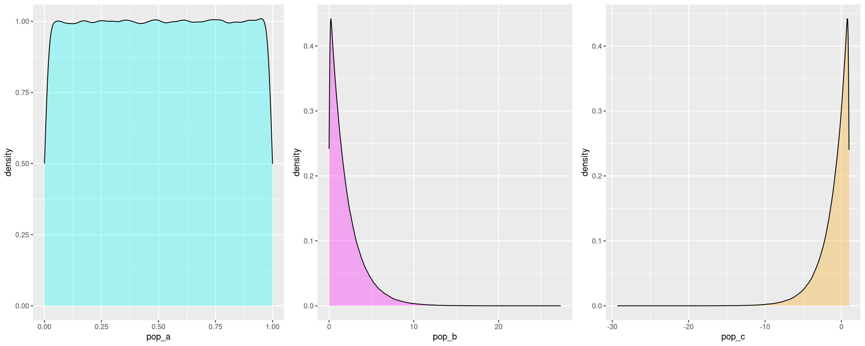

Then, we can use a function for retrieving sample means. I stored results in a list so that I could verify that the function was indeed returning what I intended (at least for small populations and a few samples; admittedly, the results get unwieldy with large populations and a large number of samples).

sample_means <- function(x, sample_size, draws) {
  ## sample size can't be larger than the population
  if (sample_size > length(x)) {
    stop("Length of x must be greater than sample_size")
  }

  ## get values as a vector
  vars <- paste0("sample_", 1:draws)

  ## create empty list
  samples <- list()

  ## could probably make this simpler with apply
  for (i in 1:draws) {
    samples[[vars[i]]] <- sample(x, sample_size, replace = TRUE)
  }

  ## get means of each sample
  means <- lapply(samples, mean) %>%
    unlist()

  ## remove names
  names(means) <- NULL

  ## get standard deviations of each sample
  standard_deviations <- lapply(samples, sd) %>%
    unlist

  ## remove names
  names(standard_deviations) <- NULL

  ## put results in a list to make it easy to inspect individual samples
  results <- list(x = x,
                  samples = samples,
                  sample_means = means,
                  standard_deviations = standard_deviations)
}

Now we can use the function on each population, taking care to use a “relatively large” sample size for each draw. Note than the sample size of each draw is not just greater than 30, it’s much greater (100,000):

draws <- 500
sample_size <- 1e5

pop_a_sample_means <- sample_means(pop_a, sample_size = sample_size, draws = draws)

pop_b_sample_means <- sample_means(pop_b, sample_size = sample_size, draws = draws)

pop_c_sample_means <- sample_means(pop_c, sample_size = sample_size, draws = draws)

After these calculations are completed, we can create density plots of the sample means:

pop_a_sample_means_dens <- ggplot(data = data.frame(x = pop_a_sample_means$sample_means), aes(x)) +
  geom_density(fill = "blue", alpha = 0.3)

pop_b_sample_means_dens <- ggplot(data = data.frame(x = pop_b_sample_means$sample_means), aes(x)) +
  geom_density(fill = "purple", alpha = 0.3)

pop_c_sample_means_dens <- ggplot(data = data.frame(x = pop_c_sample_means$sample_means), aes(x)) +
  geom_density(fill = "orange", alpha = 0.3)

grid.arrange(pop_a_sample_means_dens,
             pop_b_sample_means_dens,
             pop_c_sample_means_dens,
             nrow = 1)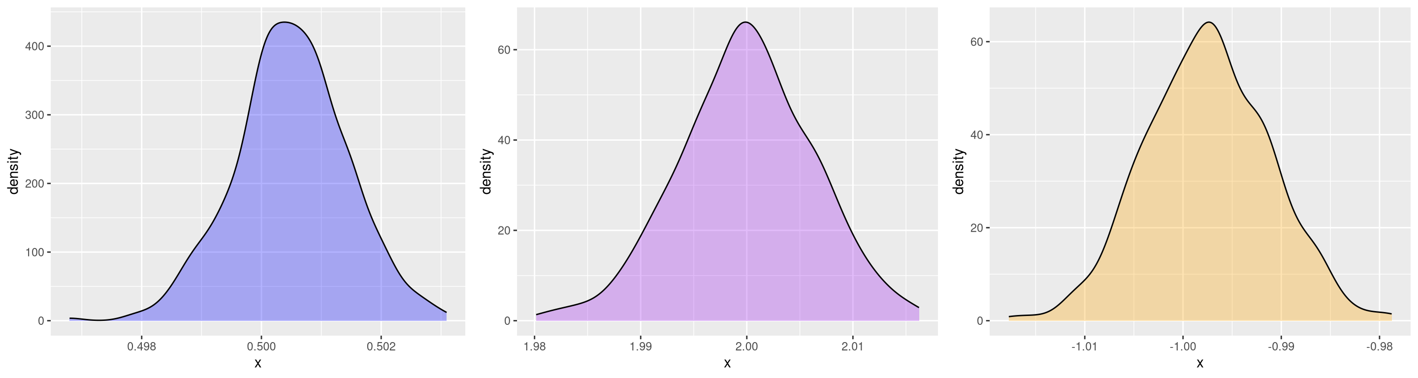

The distributions of sample means look close to normal, but after doing this quite a few times, I noticed that the skewness of the sample means of pop_b usually seemed to be positive (right-skewed) and the skewness of the sample means of pop_c usually seemed to be negative (left-skewed) and thus not actually normal.

Sure enough, calculating skewness outright, rather than just observing visually, demonstrates this to be the case:²

pop_b_skewness <- c()

for (i in 1:10) {
  skew <- sample_means(pop_b, sample_size = sample_size, draws = draws) %>%
    pluck("sample_means") %>%
    skewness()

  pop_b_skewness <- c(pop_b_skewness, skew)
}

pop_b_skewness

 [1]  0.10594045  0.06388572  0.10358930  0.31040884  0.29043669 -0.08547314
 [7]  0.23723185  0.12525226  0.03895743  0.11884991

And:

pop_c_skewness <- c()

for (i in 1:10) {
  skew <- sample_means(pop_c, sample_size = sample_size, draws = draws) %>%
    pluck("sample_means") %>%
    skewness()

  pop_c_skewness <- c(pop_c_skewness, skew)
}

pop_c_skewness

[1] -0.06902182 -0.18964411 -0.24105221 -0.16230896 -0.18134767  0.05998497
[7] -0.20168400 -0.04993342 -0.03484222 -0.23842891

While these are just a few samples and simulations, I was surprised to see this result hold for virtually all of my experiments, even when using larger population sizes, larger sample sizes, and a greater number of draws.

These simulations show that not only is it required for the samples to be “sufficiently large”, they need to be gigantic. In fact, CLT actually states that as the sampling distribution approaches infinity the sample means will converge to a normal distribution. So they need to be much, much, much larger than 30!

So what is the relevance of n ≥ 30 in statistics? This is the point at which a t-distribution approaches the normal distribution, thus making a z-test valid in that case. But it must be kept in mind that both z-tests and t-tests assume normality anyways. Put more plainly, the nefarious characteristics of a highly skewed distribution have nothing to do with the tests that consider the assumption of n ≥ 30!

The results of these simulations underscore the crucial importance of having a fundamental understanding of descriptive statistics – measures like central tendency (mean, median and mode[s]), dispersion (range, variance, standard deviation), and shape (kurtosis and skewness) in addition to using graphical measures. By understanding the significance of skewness (which is trivial to calculate in R), it led me to confirm what I suspected visually. Additionally, this experiment speaks to the way that simulations can reveal information about statistical principles.