Site Suitability/Terrain Analysis in R

In my GIS 2 class, I have students complete a simple site suitability analysis using Model Builder and ArcGIS. I’d like to have them do this through scripting, but at the time of assignment I think it’s a bit above their comfort level. I created this post as a demonstration of how to do site suitability/terrain analysis in R.

Suppose a client wants to build a cabin in Rusk County, Wisconsin and requests that it be situated situated

Below 1200 ft.
On a slope of less than 3 degrees
Facing northeast, east, or southeast (angle between 22.5 and 157.5 degrees)

First, we will load packages then download and unzip the DEM data.

library(here)
library(tigris)
library(raster)
library(dplyr)
library(sf)
library(measurements)
library(leaflet)

## download dem and use the "here" package to set a "relative" working directory
download.file("https://gitlab.com/mhaffner/data/raw/master/DEM_30m.zip",
              destfile = here("data/DEM_30m.zip"))
## unzip dem data
unzip(here("data/DEM_30m.zip"), exdir = here("data"))

## load dem
wi.dem <- raster(here("data/DEM_30m/demgw930/"))

plot(wi.dem)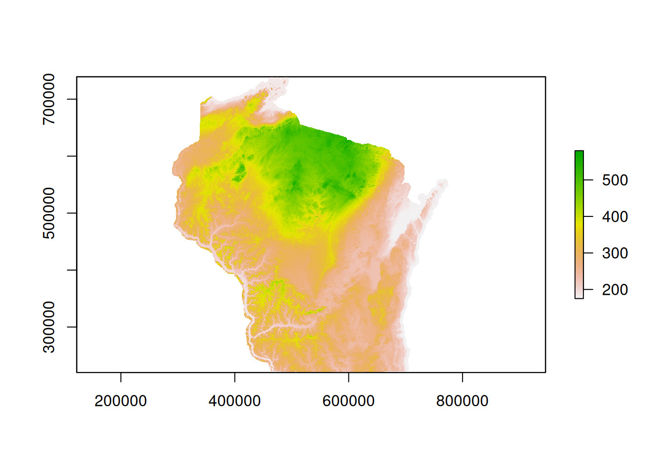

Next, we will download county data for Wisconsin, extract just Rusk County, and transform the CRS into that of the DEM.

## use sf instead of sp, use cartographic boundary files since they look nicer
rusk.co <- counties("55", class = "sf", cb = TRUE, progress_bar = FALSE) %>%
  filter(NAME == "Rusk") %>%
  st_transform(., crs(wi.dem))

After this, we can crop the DEM to the county boundary since everything outside of Rusk County is irrelevant.

## crop dem to country boundaries
rusk.dem <- crop(wi.dem, rusk.co)

plot(rusk.dem, main = "Rusk County DEM")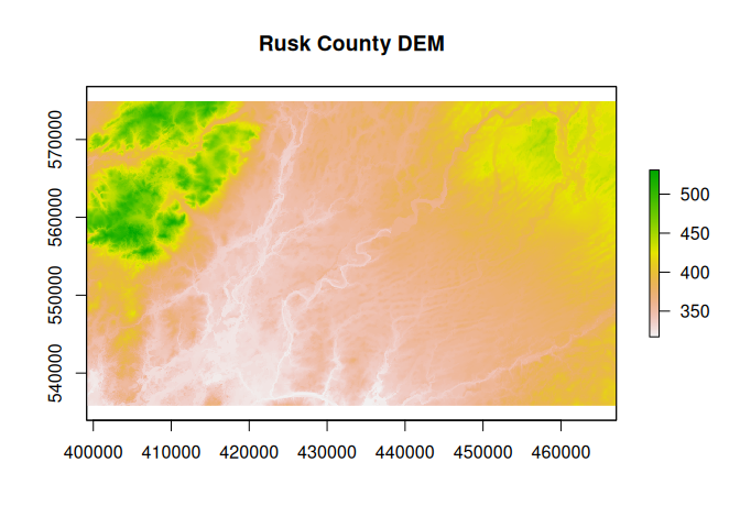

Next, we are ready to implement terrain analysis functions and complete the binary site suitability analysis. We can simply use the < operator to get all cells under 1200 ft. Then, we can “chain” the other functions together using the & operator. Here, we can use the terrain function and specify the opt argument.

rusk.suit <-
  ## elevation; under 1200 ft, convert to m (units of the dem)
  rusk.dem < conv_unit(1200, "ft", "m") &
  ## aspect; between 22.5 and 157.5 degrees
  terrain(rusk.dem, opt = "aspect", unit = "degrees") > 22.5 &
  terrain(rusk.dem, opt = "aspect", unit = "degrees") < 157.5 &
  ## slope; less than 3 degrees
  terrain(rusk.dem, opt = "slope", unit = "degrees") < 3

plot(rusk.suit)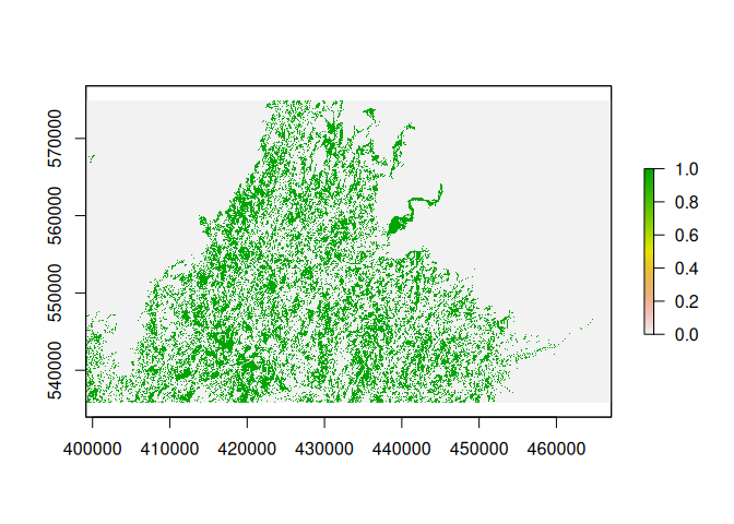

Of course, the individual criteria may be of interest on their own. If that is the case, then we can create a function that completes each operation within its own plot function and displays each criteria individually.

plot_criteria <- function(elev, asp.min, asp.max, slope) {
  ## get plot parameters so we can reset them after plotting is done
  opar <- par()

  ## set plot parameters
  par(mfrow = c(2,2))

  ## plot each step
  plot(rusk.dem, main = "DEM")
  plot(rusk.dem < conv_unit(elev, "ft", "m"), main = "Elevation criteria",
       col = c("#ffffff", "#0000ff"))
  plot(terrain(rusk.dem, opt = "aspect", unit = "degrees") > asp.min &
       terrain(rusk.dem, opt = "aspect", unit = "degrees") < asp.max, main = "Aspect criteria")
  plot(terrain(rusk.dem, opt = "slope", unit = "degrees") < slope, main = "Slope criteria",
       col = c("#ffffff", "#ff9900"))

  ## reset plot parameters
  par(opar)
}

plot_criteria(1200, 22.5, 157.5, 3)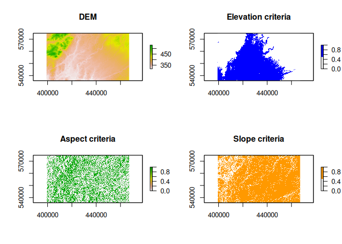

It would also be nice to visualize the final result with some context. To do this, we can use a leaflet basemap.

leaflet(width = "100%") %>%
  addTiles() %>%
  addRasterImage(rusk.suit, opacity = 0.5, col = c("#ffffff", "#ff0000"))

From here, it’s clear that a significant portion of the suitable area is in water which is probably not ideal. Then again, maybe so if the client is open to a boat cabin!