Introduction

Anyone who listens to Gundy’s press conferences around signing day or reads Pistols Firing Blog (PFB) articles on recruiting (and their corresponding comments) knows that Oklahoma State Football’s recruiting practices are heavily scrutinized. The writers of PFB have pointed out that Gundy’s attitude toward recruiting has seemingly changed. Where the mantra used to be “recruiting is the most important thing we do,” it now seems less important. With Gundy’s recent contract extension and apparent nonchalant attitude toward the disappointing results of the 2018 season, some have accused the head coach of becoming complacent, particularly in the area of recruiting. Though Oklahoma State has historically over-performed based on its recruiting class rankings, the probability of success is lower with less talented players. As a geographer, I naturally wonder how the locational aspects of Oklahoma State’s recruiting practices have changed over time, and that’s what I’ll be discussing in this piece.

Rather than making a prediction beforehand about how changes have occurred, (e.g., Gundy has become less effective in recruiting within the region, or, on the other hand, the geographic variability has lessened over time) my approach is more exploratory. I’m simply looking for an observable inflection point – or consistent changes over time – that help explain how Gundy’s recruiting practices have changed with his apparent change in attitude.

Before I begin, I must make a few disclaimers. First, a change in the spatial practices of OSU recruits does not mean lower quality athletes, and my approach does not consider recruits’ rankings. Few people would complain if OSU only signed players from Texas… if those players all happened to be the top 20-ish in the state, or if OSU landed zero players within a 500 miles radius of Stillwater but received all four and five star recruits from California, Washington, New York, and Florida. Additionally, recruiting isn’t all on Gundy - it’s a group effort among all coaches, and assistants can have considerable influence in where players sign (e.g., consider Marcus Arroyo’s influence).

That said, recruiting starts with the head coach, and caveats aside, geography clearly matters. Virtually every university signs more recruits from near than far, and Oklahoma State faces considerably different recruiting challenges than other similarly sized schools in other parts of the country (e.g., Washington State, Clemson, or Boise State). Conference alignment, proximity to other universities, recruits’ distance from family and friends, the weather, culture, and other personal factors related to location all matter. My colleagues who are Nebraska alums bemoan the Huskers’ de-emphasis on local recruiting that began in the early 2000s – which some blame for Nebraska’s downfall – and it’s hard to ignore the coincident struggles that Nebraska, Missouri, and Colorado have all faced since leaving the Big XII.

The spatialities of recruiting have mostly been beaten like a dead horse in the world of sports geography, so I wanted to do something a bit unconventional by investigating more than just the locations of where recruits come from. In this piece I explore (1) change by year over Gundy’s entire tenure, (2) measures of central spatial tendency like the mean and median center, (3) a measure of dispersion (i.e. standard deviation of distance from Stillwater), and (4) interactive visualizations through web maps. For all analyses and visualization I use the R Project for Statistical Computing, and I retrieved data on Oklahoma State’s recruits from Rivals.com. If you’re interested in the technical aspects or source code, you can read about them here.

All recruits

First, I map the hometowns (or in the case of transfers, previous locations) of all signees recruited during Gundy’s tenure, with 2005 excluded since the players during this year were not his recruits. Note: each year is a selectable layer, so feel free to explore!

The majority of recruits outside of Oklahoma come from Texas (no surprise), particularly Dallas, Houston, and the eastern half of the state. On one hand this seems to be simply an artifact of proximity to major population centers (i.e. Dallas and Houston), yet there is an apparent disproportionate number of recruits from Texas (and Kansas) compared to Arkansas or Missouri. Of course, there is not a one-to-one correspondence between population and quality of football recruits though. Outside of Oklahoma’s bordering states, several small clusters can be seen near Atlanta, southern Louisiana and Mississippi, and southern California.

Central tendency and dispersion

The field of spatial statistics exists in part because humans are notoriously bad at recognizing spatial patterns. Though this web map is fun to play with and displays general distributions, it doesn’t tell us anything definitive about patterns over time. Rather than just eyeballing recruits locations year-to-year, I assess trends using two measures of central tendency for spatial data – the mean and median center – and a measure of dispersion: standard deviation of distance from Stillwater.

Mean and median centers are calculated as one would expect, except utilizing two dimensions (latitude and longitude) instead of one. Rather than comparing these separately, I think they are useful to view together. Medians reduce the influence of outliers, which in this case are introduced by intermittent recruits from California, the Northeast, and Canada. Chuba Hubbard’s hometown, for example, lies at a whopping 53.5 degrees north.

In many cases – especially when underlying distributions are not assessed first – the median is a more appropriate measure, yet both measures yield similar results in this case. The median center does reduce the amount of east-west variability, however, and makes 2009 and 2016 stand out from the other years. Aside from these years, the centers appear to remain remarkably stable, including recent years (2017 - 2019), with no apparent systematic change over time.

It’s hard to ignore that many of the 2009 recruits played for the historic 2011 team several years later, yet the results two years following 2016 (i.e. 2018) were quite different from 2011. Being able to tie individual recruiting classes directly to performance in future seasons would be a luxury, but unfortunately I don’t think it works way. Unlike basketball in which one superb recruiting class can drastically alter a team’s trajectory, football is different. Success is made out of pattern of high caliber recruiting over long periods of time.

Dispersion

While informative, these measures do not consider dispersion or within-year variability. For example, if Oklahoma State received all of its recruits from Dallas during one year and zero recruits from Dallas during another year, the two years could still have the exact same mean or median center (that said, 2009 and 2016 have similarly dispersed patterns compared to other years). Next, I create a plot showing the distance and direction of each recruit’s hometown to Stillwater by year.

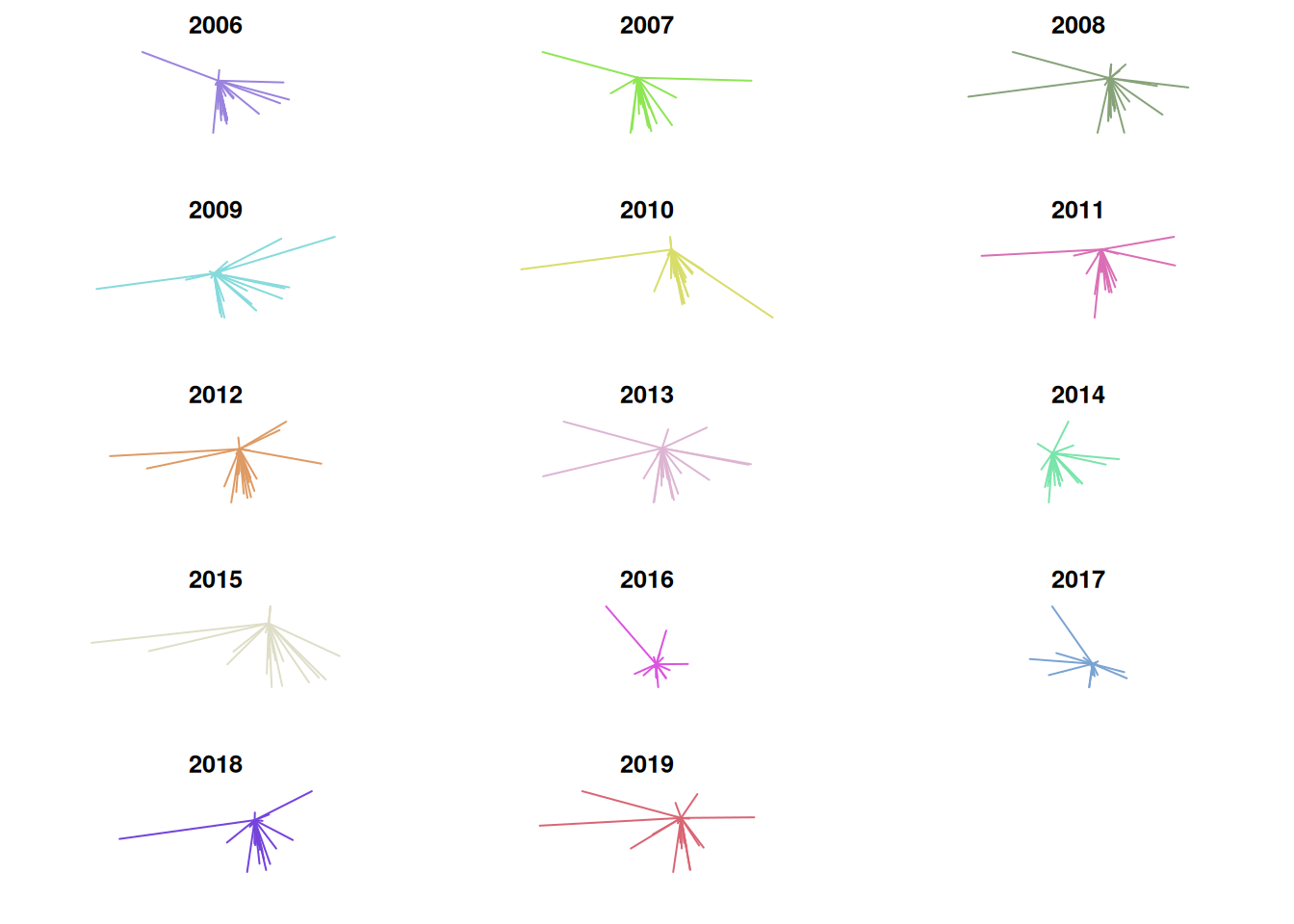
This plot displays some intriguing patterns. In each of the years 2007, 2010, and 2011 Oklahoma State signed only one player from north of Stillwater (2015 appears this way too, but actually two signees came from El Dorado, KS), emphasizing the importance of Texas – and other parts of the southern US – to its recruiting efforts. Next, I create a plot comparing mean, median, and standard deviation of distance from Stillwater.

Again, no systematic trends appear, although the median distance from Stillwater is less in 2016 - 2019 than any previous years. That said, standard deviation is not less during these years; in fact, 2017 has the greatest standard deviation in the dataset (largely thanks to Chuba Hubbard).

Conclusion

So what does all of this mean? I think the most straightforward takeaway is that the geography of Oklahoma State’s recruiting practices has remained fairly stable over Gundy’s tenure. If Gundy has become complacent, it’s not appearing in locational distributions of recruits. That said, recruiting efforts could certainly be improved, and there is one glaringly relevant takeaway to the future of Oklahoma State football: the array of locations from which players come is good enough in that there are plenty of sufficiently talented players in those places. The challenge is recruiting better players from those locations. As mentioned earlier, this assessment did not consider recruits’ high school (or JUCO) ratings.

While it is a bit disappointing to not find something juicier, there are several logical ways this small project could be extended. First and foremost, the effect of distance on the quality of recruits may be revealing. For example, are signees from farther away rated lower than those close to Stillwater? If so, this may give some credence to the idea that “it’s difficult to get players to come to Stillwater” or, more precisely, that “Oklahoma State is less successful is getting good players from far away to come to Stillwater.” Of course, this assumes current conditions with the present efforts and strategies put into recruiting. On the flip side, if results were insignificant (i.e. distance does not have an effect on the quality of recruits), perhaps Oklahoma State could be more aggressive – and confident – in offering scholarships to higher rated recruits from farther away. These effects could be assessed with a simple correlation analysis.

What could be even more informative, however, is a comparative study with another university – either one in the Big XII, similarly positioned regionally¹, or a comparatively sized university in another part of the country. With the recent comparisons of Oklahoma State to Clemson, a side-by-side comparison of these two universities’ geographies of recruiting may make for a fascinating study.

If you catch something that I didn’t see in the data or if you have another idea for a follow-up study, feel free to point it out in the comments!

Footnotes